
CXC Home | Search | Help | Image Use Policy | Latest Images | Privacy | Accessibility | Glossary | Q&A
Introduction:
The ice sheets in the Polar Regions retain signatures of the atmospheric conditions at the time each annual layer of snow was deposited. Snow falling in the interior Polar Regions and Greenland, above the summer melt boundary, is compacted and incorporated into the ice sheets unless major climatic change causes melting. Ice core samples from the ice sheets in the Polar Regions, therefore, contain information about past climatic and environmental conditions.
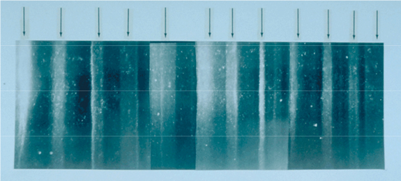
Figure 1. A 19 cm long section of the GISP2 ice core from a depth of 1855 m showing annual layer structure illuminated from below by a fiber optic source. The section contains 11 annual layers with the summer layers (arrowed) sandwiched between the darker winter layers.
This investigation involves examining the liquid electrical conductivity and nitrate concentration data from a 122-meter ice core collected from the Greenland ice sheet in 1992. The upper 12 meters of the least compacted GISP2 H-core – called firn - were analyzed on-site in Greenland. The remaining core was sent to the National Ice Core Laboratory in Denver, Colorado. At the lab, the core was sliced into 1.5 cm thick samples, and then each sample was inserted into a glass vial which was sealed and stored at -24oC. The vials were removed from storage and allowed to melt at room temperature for one hour. The liquid samples were removed from the vials with a syringe and injected into a UV absorption cell (UV spectrophotometer) to determine the nitrate values in absorption units.
Nitrates (NO3–) are one of the major anions found in snow. Nitrate deposition results from reactions in the atmosphere between nitrogen oxides (NOx), ozone (O3), and the hydroxyl radical (OH–). The terrestrial sources of nitrogen oxides are the burning of fossil fuels and biomass burning, emissions from soil produced by living organisms, and lightning. Nitrogen oxides react with water to form nitric acid (HNO3). Extra-terrestrial sources of high energy particles and radiation penetrate the earth at the magnetic poles, ionizing the atmosphere and forming nitrates. Gravitational nitrate fallout from the atmosphere, either by dry deposition or falling snow, results in nitrate deposition onto the surface. The nitrate record is important in studying long-term climate change and solar sunspot activity.
After the nitrate values were obtained from the UV spectrophotometer, the samples were inserted directly into a micro-conductivity cell to measure the conductivity in micro Siemens per centimeter (μS/cm). The liquid electrical conductivity measurements (LEC) measure the change in all acidic ions, including nitrate ions, along the length of the core. An increase in acidity results in an increase in conductivity. A high concentration of alkaline dust in the ice reduces the acidity and therefore the conductivity.
A. Dating Ice Core Samples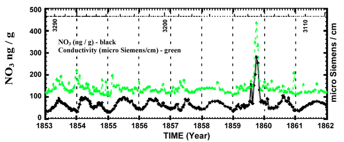
Figure 2. A section of perfectly correlated high-resolution nitrate and electrical conductivity data from the Greenland ice core record for the years1561-1994. Numbers along the top, 3290, 3200, and 3110 refer to the sample number.
Nitrate concentrations show an annual background variation. Examine the graph of nitrate concentration (in black) in Figure 2 above. The vertical dotted line goes through January 1st for each year. (The assumption is that the lowest point in the seasonal signal occurs at the depth of winter.)
1. Is there evidence for seasonal variations in nitrate concentrations?
2. Referring back to the main sources of nitrogen oxides in the atmosphere in the introduction, what might cause these seasonal variations? Explain.
On the horizontal axis of Plate 1a Nitrate and Conductivity Record, GISP-H-Part I the numbers correspond to the sample number. Sample 0.0 was taken from the top of the ice core. This sample is from the most recent layer deposited, which corresponds to the year 1992 when the core was collected.
3. In the first section (samples 0.0 to 1999.0), at what sample number does an overall increase in the nitrate concentration occur that might correspond to human related activity? Use the seasonal nitrate variation to approximate the year that human activity resulted in increased nitrate deposits.
B. The Conductivity Record & Volcanic Eruptions4. This activity is designed for four teams. Each team will analyze a graph of one quarter of the ice core record (~2000 samples). Note: Moving from left to right, the graphical data extends further back in time.
| team | sample#'s |
| 1 | 0.0 – 1999.0 |
| 2 | 2000.0 – 3999.0 |
| 3 | 4000.0 – 5999.0 |
| 4 | 6000.0 – 7800.0 |
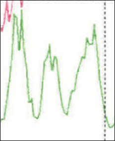
Figure3. Seasonal variation in the nitrate cycle spanning ~3 years
5. Each team (except Team 2) will be given a sample range and the eruption date of an Icelandic volcano. Mark the conductivity anomaly associated with this eruption (including name and date). Note the accompanying drop in nitrate concentration for this conductivity anomaly.
6. Continue to mark the conductivity anomalies for the remaining volcanoes using the corresponding table for your team. To help with this task, the conductivity value is given in the last column. The seasonal nitrate cycle can be used to help count years (see figure 3). Icelandic volcanoes, which are geographically close to the ice core collection site in Greenland are in bold print.
Team 1 - Volcanic Eruptions (samples 0.0 – 1999.0)
Mark the conductivity anomaly associated with the eruption of the Icelandic volcano Hekla in 1970 (between samples 600.0 and 700.0) on your graph.
| year of volcanic event | name | conductivity in ice core μs cm–1 X 10⁻² |
| 1986 | Augustine | 290 |
| 1977 | Sakura-Jima | 270 |
| 1970 | Hekla | 410 |
| 1969 | Sheveluch | 250 |
| 1961 | Askja | 190 |
| 1947 | Hekla | 380 |
| 1924 | Raikoke | 220 |
| 1918 | Katla | 260 |
Team 2 - Volcanic Eruptions (samples 2000.0 – 3999.0)
None of the volcanoes in the table below are nearby, Icelandic volcanoes. Instead mark the nitrate and conductivity anomaly corresponding to Carrington’s White Flare in 1859 between samples 3100.0 and 3200.0 on the graph. The flare will be discussed further in part 3 of this activity.
| year of volcanic event | name | conductivity in ice core μs cm–1 X 10⁻² |
| 1912 | Katmai | 250 |
| 1885 | White River Ash | 200 |
| 1883 | Krakatau | 240 |
| 1854 | Sheveluch | 220 |
| 1853 | Chikurachki-Tatarinov | 190 |
| 1835 | Cosigüina | 200 |
| 1831 | Babuyan Claro | 210 |
| 1815 | Tambora | 270 |
Team 3 - Volcanic Eruptions (samples 4000.0 – 5999.0)
Mark the conductivity anomaly associated with the eruption of the Icelandic volcano Laki in 1783 (between samples 4500.0 and 4600.0) on the graph.
| year of volcanic event | name | conductivity in ice core μs cm–1 X 10⁻² |
| 1801 | Mt. St. Helens | 170 |
| 1783 | Laki | >450 |
| 1739 | Tarumai | 230 |
| 1728 | Krafla* | 210 |
| 1727 | Oraefajoküll | 280 |
| 1724 | Mývatn Fire | 220 |
| 1721 | Katla | 190 |
| 1693 | Hekla | 250 |
Team 4 - Volcanic Eruptions (samples 6000.0 – 7800.0)
Mark the conductivity anomaly associated with the eruption of the Icelandic volcano Tarumai in 1667 (between samples 6300.0 and 6400.0) on the graph.
| year of volcanic event | name | conductivity in ice core μs cm–1 X 10⁻² |
| 1667 | Tarumai | 400 |
| 1660 | Katla | 290 |
| 1630 | Furnas | 290 |
| 1625 | Katla | 260 |
| 1597 | Helka | 260 |
C. The Nitrate Record & Solar Flares
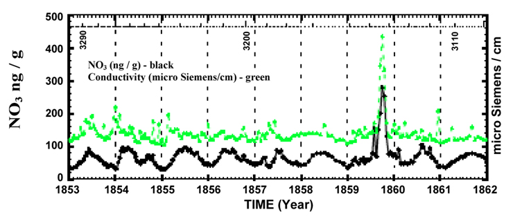
Figure 2. A section of perfectly correlated high-resolution nitrate and electrical conductivity data from the Greenland ice core record for the years1561-1994. Numbers along the top, 3290, 3200, and 3110 refer to the sample number.
7. Examine Figure 2 above and note the interruption of the annual nitrate variation by two impulsive events. The second is the largest event in the entire Greenland core nitrate record 1561–1991. Well-known time markers from the 1853 and 1854 eruptions of Sheveluch and Chikurachki-Tatarinov help determine the date of this nitrate anomaly. Team 2 has already labeled this event on their section of the GISP ice core record. What is the date of this event?
8. Read the excerpt from “A Super Solar Flare” on the following page. How does the date of this event correspond to the nitrate anomaly identified above?
9. Record the dates on your section of the ice core record of nitrate anomalies that may correspond to solar proton events. [Note: The tables include the nitrate concentration value of the peak that has been identified by scientists as corresponding to these events.] The ice core section for Team 4 does not contain any data for solar proton events during this time; team 4 can work with one of the other teams.
10. The complete record also includes two time periods of known low solar activity, the Dalton (1833–1798) and Maunder (1715–1645) Minima which can be marked if your section of the ice core graph includes these dates.
11. When all the groups have finished identifying the solar proton events, tape the four sections of the ice core record together to form one long strip.
Excerpt from "A Super Solar Flare"—Science@ NASA, May 6, 2008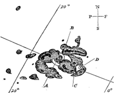
Sunspots sketched by Richard Carrington on Sept. 1, 1859. Copyright: Royal Astronomical Society
At 11:18 AM on the cloudless morning of Thursday, September 1, 1859, 33-year-old Richard Carrington—widely acknowledged to be one of England's foremost solar astronomers—was in his well-appointed private observatory. Just as usual on every sunny day, his telescope was projecting an 11-inch-wide image of the sun on a screen, and Carrington skillfully drew the sunspots he saw.
On that morning, he was capturing the likeness of an enormous group of sunspots. Suddenly, before his eyes, two brilliant beads of blinding white light appeared over the sunspots, intensified rapidly, and became kidney-shaped. Realizing that he was witnessing something unprecedented and "being somewhat flurried by the surprise," Carrington later wrote, "I hastily ran to call someone to witness the exhibition with me. On returning within 60 seconds, I was mortified to find that it was already much changed and enfeebled." He and his witness watched the white spots contract to mere pinpoints and disappear.
It was 11:23 AM. Only five minutes had passed.
Just before dawn the next day, skies all over planet Earth erupted in red, green, and purple auroras so brilliant that newspapers could be read as easily as in daylight. Indeed, stunning auroras pulsated even at near tropical latitudes over Cuba, the Bahamas, Jamaica, El Salvador, and Hawaii.
Even more disconcerting, telegraph systems worldwide went haywire. Spark discharges shocked telegraph operators and set the telegraph paper on fire. Even when telegraphers disconnected the batteries powering the lines, aurora-induced electric currents in the wires still allowed messages to be transmitted.
"What Carrington saw was a white-light solar flare—a magnetic explosion on the sun," explains David Hathaway, solar physics team lead at NASA's Marshall Space Flight Center in Huntsville, Alabama.
Team 1 – Solar Proton Events
|
Team 2 – Solar Proton Events End of Dalton Minima – 1833
*Carrington’s White Flare (previously marked on the graph) |
||||||||||||||||||||||||||||||||||||||||||||||||||||||||||||
Team 3 – Solar Proton Events Start of Dalton Minima – 1798 End of Maunder Minima – 1715
|
Team 4 – Solar Proton Events Start of Maunder Minima – 1645 |
D. Ice Core Record & Historic Supernovas
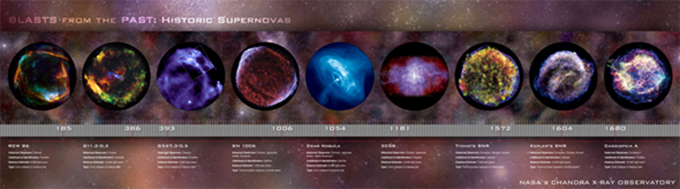
12. Are there nitrate anomalies in the GISP2 H-core record that might correspond to the historic supernovas Tycho and Kepler? Two methods to date the anomalies are:
- A count of the seasonal nitrate cycles from a known date.
- Select two labeled dates from the ice core graph on either side of the date of the suspected supernova nitrate spike. Measure the distance between these two peaks in cm and use the measurement to calculate a scale in cm/year to determine the dates of the nitrate anomalies more accurately.
Discuss the accuracy of each of these methods.
13. Read "Did John Flamsteed Observe the Supernova, Cas A?" on page 9. Is there a nitrate anomaly that might correspond to either 1680 or 1667? Label and date the anomaly.
Supernova Data Table
| name and date of historic supernova | sample # of possible corresponding nitrate anomaly |
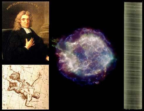
Did John Flamsteed Observe the Supernova, Cas A?
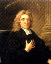
John Flamsteed
John Flamsteed was the first Royal Astronomer of England. His observations were published posthumously. The earlier observations, made by using a sextant, were printed in Halley’s 1712 edition of the Historia coelestis, and reappeared in the little-used volume i of the 1725 edition. And though the catalog was a major achievement, it was marred by errors of observation and computation. Caroline Herschel compiled an Index to Flamsteed’s observations. She noted that Flamsteed had twice observed a star that he designated as 3 Cassiopeiae, and since no star was located at the coordinates he had calculated, Herschel decided Flamsteed’s calculations were erroneous and substituted 3 Cassiopeiae for the nearby star AR Cassiopeiae which was in the same location as her recalculated values for the coordinates for 3 Cassiopeiae. Francis Baily, picking up where Caroline Herschel left off, was not satisfied with her resolution of the problem with 3 Cassiopeiae. Since the actual observational data for reducing the coordinates for 3 Cassiopeiae were not written down, Baily excluded the star from the British Association catalogue which was published in 1845.
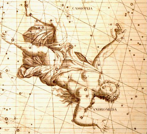
Historia Coelestis, 1725
However, the observation may have been there all along. Caroline Herschel did not see it because she compiled her Index to volume ii of the Historia coelestis, which contains data collected after 1689. Francis Baily did come across the observation, but did not recognize the significance and ignored the information. In volume i of Halley’s 1712 edition of the Historia coelestis, on the night of August 16th, 1680, John Flamsteed observed a star that he designated as “supra τ”. Flamsteed had used Scheat (β Pegasi) and Algol (β Persei) to determine the location of supra τ. The newly observed star, supra τ then became 3 Cassiopeiae in the 1725 catalog. On the section of the Cassiopeia plate in Bevis’s star atlas, c. 1750, the Flamsteed numbers and letter designations have been added. The position of Cas A is indicated by a small circle (also added) just to the left of 3 Cassiopeiae (formerly noted as supra τ.) The prominent object at the bottom center is Tycho’s supernova of 1572.
If this analysis is correct, then high energy photons from the supernova collapse reached earth in August of 1680 and were observed by John Flamsteed. However, if the age of the event is measured from the expansion rate of the remnant, the calculated age of the event is 1667 – matching the nitrate anomaly in the ice core. The interpretations of the historical record are subjective and not conclusive – as are the complexities of analyzing the nitrate record in ice cores. With the ever-increasing sophistication of supernovae modeling and ice core data extraction, maybe one day the age of Cas A will be determined and no longer remain a mystery!
Extensions:
14. Several of the peaks in the nitrate concentration and liquid conductivity spikes have not been identified. What other terrestrial or extra-terrestrial events could lead to significant deposition of nitrates? Research the following:
- Novaya Zemlya testing of Tsar Bomba, literally the "Emperor Bomb", and the Western name for the RDS-220 hydrogen bomb—the largest, most powerful nuclear weapon ever detonated.
- Tunguska Event, a massive explosion that occurred near the Podkamennaya (Lower Stony) Tunguska River in what is now Krasnoyarsk Krai of Russia.
Write a paragraph describing the event (include the date it occurred). Find peaks in the nitrate concentration and/or liquid conductivity curves that could correspond to these events. Explain your reasoning.
15. Choose other conductivity and nitrate anomalies to date and research possible corresponding events. Present the findings, citing references.
Back to Ice Core Index
Revised: January 08, 2013